what is the potential v0 in the limit as h goes to zero?
7.four: Calculations of Electric Potential
- Page ID
- 4388
Learning Objectives
By the stop of this department, you will be able to:
- Summate the potential due to a point accuse
- Calculate the potential of a system of multiple signal charges
- Describe an electric dipole
- Ascertain dipole moment
- Calculate the potential of a continuous charge distribution
Point charges, such as electrons, are among the fundamental building blocks of thing. Furthermore, spherical charge distributions (such equally accuse on a metal sphere) create external electric fields exactly similar a point accuse. The electrical potential due to a bespeak charge is, thus, a example we need to consider.
Nosotros can employ calculus to observe the work needed to movement a test charge q from a large distance away to a distance of r from a betoken charge q. Noting the connection between work and potential \(Due west = -q\Delta V\), equally in the last section, nosotros can obtain the following result.
Electric Potential \(V\) of a Point Charge
The electric potential \(V\) of a betoken accuse is given by
\[\underbrace{V = \dfrac{kq}{r}}_{\text{point charge}} \label{PointCharge}\]
where \(k\) is a constant equal to \(9.0 \times x^ix \, N \cdot m^2/C^2\).
The potential in Equation \ref{PointCharge} at infinity is chosen to exist zero. Thus, \(V\) for a indicate charge decreases with distance, whereas \(\vec{E}\) for a point charge decreases with distance squared:
\[E = \dfrac{F}{q_t} = \dfrac{kq}{r^ii}\]
Recall that the electric potential 5 is a scalar and has no direction, whereas the electric field \(\vec{E}\) is a vector. To find the voltage due to a combination of point charges, you add together the individual voltages equally numbers. To find the total electric field, y'all must add the private fields as vectors, taking magnitude and direction into account. This is consistent with the fact that 5 is closely associated with energy, a scalar, whereas \(\vec{East}\) is closely associated with force, a vector.
Instance \(\PageIndex{1}\): What Voltage Is Produced by a Small Accuse on a Metal Sphere?
Charges in static electricity are typically in the nanocoulomb (nC) to microcoulomb \((\mu C)\) range. What is the voltage five.00 cm abroad from the middle of a i-cm-diameter solid metal sphere that has a –3.00-nC static accuse?
Strategy
As we discussed in Electric Charges and Fields, charge on a metal sphere spreads out uniformly and produces a field like that of a indicate accuse located at its heart. Thus, nosotros can observe the voltage using the equation \(V = \dfrac{kq}{r}\).
Solution
Inbound known values into the expression for the potential of a bespeak charge (Equation \ref{PointCharge}), we obtain
\[\begin{align} V &= k\dfrac{q}{r} \nonumber \\[4pt] &= (9.00 \times 10^ix \, N \cdot m^2/C^2)\left(\dfrac{-iii.00 \times 10^{-ix}C}{5.00 \times 10^{-2}m}\correct) \nonumber \\[4pt] &= - 539 \, V. \nonumber \end{align} \nonumber \]
Significance
The negative value for voltage means a positive charge would be attracted from a larger distance, since the potential is lower (more than negative) than at larger distances. Conversely, a negative charge would exist repelled, equally expected.
Example \(\PageIndex{ii}\): What Is the Excess Charge on a Van de Graaff Generator?
A demonstration Van de Graaff generator has a 25.0-cm-bore metallic sphere that produces a voltage of 100 kV virtually its surface (Effigy). What excess charge resides on the sphere? (Assume that each numerical value hither is shown with iii significant figures.)
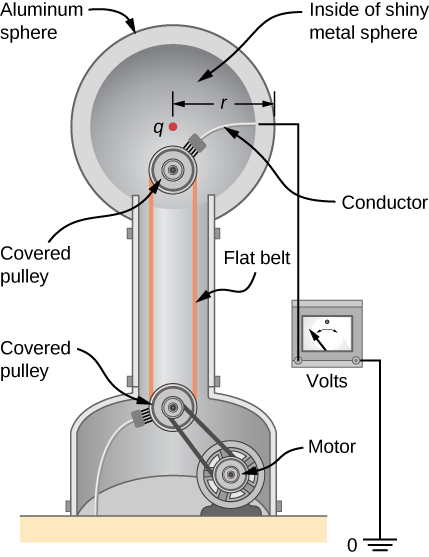
Strategy
The potential on the surface is the same equally that of a bespeak charge at the eye of the sphere, 12.5 cm away. (The radius of the sphere is 12.v cm.) We tin thus determine the backlog charge using Equation \ref{PointCharge}
\[V = \dfrac{kq}{r}.\]
Solution
Solving for \(q\) and entering known values gives
\[\begin{align} q &= \dfrac{rV}{k} \nonumber \\[4pt] &= \dfrac{(0.125 \, m)(100 \times x^3 \, V)}{8.99 \times ten^9 N \cdot m^two/C^two} \nonumber \\[4pt] &= 1.39 \times x^{-6} C \nonumber \\[4pt] &= one.39 \, \mu C. \nonumber \end{align} \nonumber \]
Significance
This is a relatively small charge, but information technology produces a rather big voltage. Nosotros have another indication hither that information technology is hard to store isolated charges.
Exercise \(\PageIndex{one}\)
What is the potential inside the metal sphere in Example \(\PageIndex{1}\)?
Solution
\[\begin{align} V &= k\dfrac{q}{r} \nonumber \\[4pt] &= (viii.99 \times 10^nine Northward \cdot g^two/C^2) \left(\dfrac{-3.00 \times ten^{-ix} C}{5.00 \times ten^{-3} g}\right) \nonumber \\[4pt] &= - 5390 \, 5\nonumber \end{align} \nonumber \]
Recall that the electric field within a conductor is zippo. Hence, whatsoever path from a indicate on the surface to any point in the interior volition take an integrand of zero when calculating the change in potential, and thus the potential in the interior of the sphere is identical to that on the surface.
The voltages in both of these examples could exist measured with a meter that compares the measured potential with basis potential. Ground potential is oftentimes taken to be zippo (instead of taking the potential at infinity to be zero). It is the potential divergence between two points that is of importance, and very often there is a tacit supposition that some reference point, such every bit Globe or a very afar point, is at zero potential. As noted before, this is analogous to taking sea level equally \(h = 0\) when considering gravitational potential energy \(U_g = mgh\).
Systems of Multiple Point Charges
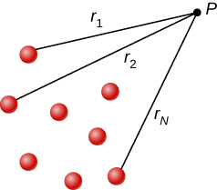
Just as the electric field obeys a superposition principle, so does the electric potential. Consider a organisation consisting of N charges \(q_1,q_2,. . ., q_N\). What is the net electric potential 5 at a space signal P from these charges? Each of these charges is a source charge that produces its own electric potential at bespeak P, contained of whatever other changes may be doing. Allow \(V_1, V_2, . . ., V_N\) be the electric potentials at P produced by the charges \(q_1,q_2,. . ., q_N\), respectively. And then, the cyberspace electrical potential \(V_p\) at that point is equal to the sum of these individual electric potentials. You can easily show this by calculating the potential free energy of a exam charge when yous bring the examination charge from the reference betoken at infinity to betoken P:
\[V_p = V_1 + V_2 + . . . + V_N = \sum_1^N V_i.\]
Note that electric potential follows the aforementioned principle of superposition equally electric field and electrical potential energy. To bear witness this more explicitly, note that a test charge \(q_i\) at the indicate P in space has distances of \(r_1,r_2, . . . ,r_N\) from the N charges fixed in space in a higher place, as shown in Figure \(\PageIndex{ii}\). Using our formula for the potential of a signal charge for each of these (causeless to be point) charges, we notice that
\[V_p = \sum_1^N k\dfrac{q_i}{r_i} = chiliad\sum_1^N \dfrac{q_i}{r_i}. \characterization{eq20}\]
Therefore, the electric potential energy of the test accuse is
\[U_p = q_tV_p = q_tk\sum_1^N \dfrac{q_i}{r_i},\] which is the same as the work to bring the test charge into the organisation, as found in the outset department of the chapter.
The Electric Dipole
An electrical dipole is a organisation of two equal just opposite charges a stock-still distance apart. This system is used to model many real-earth systems, including atomic and molecular interactions. One of these systems is the water molecule, under certain circumstances. These circumstances are met inside a microwave oven, where electric fields with alternating directions make the h2o molecules change orientation. This vibration is the same every bit heat at the molecular level.
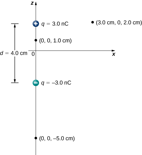
Case \(\PageIndex{3}\): Electric Potential of a Dipole
Consider the dipole in Figure \(\PageIndex{iii}\) with the charge magnitude of \(q = three.0 \, \mu C\) and separation altitude \(d = 4.0 \, cm.\) What is the potential at the post-obit locations in space? (a) (0, 0, i.0 cm); (b) (0, 0, –5.0 cm); (c) (3.0 cm, 0, 2.0 cm).
Strategy
Employ \(V_p = k \sum_1^N \dfrac{q_i}{r_i}\) to each of these three points.
Solution
a. \(V_p = m \sum_1^Northward \dfrac{q_i}{r_i} = (ix.0 \times 10^9 \, Northward \cdot grand^two/C^two) \left(\dfrac{3.0\space nC}{0.010 \, k} - \dfrac{iii.0\space nC}{0.030 \, thousand}\right) = i.eight \times 10^iii \, Five\)
b. \(V_p = 1000 \sum_1^Due north \dfrac{q_i}{r_i} = (nine.0 \times ten^ix \, N \cdot m^2/C^2) \left(\dfrac{3.0\space nC}{0.070 \, yard} - \dfrac{3.0\infinite nC}{0.030 \, m}\correct) = -5.1 \times ten^2 \, V\)
c. \(V_p = thousand \sum_1^N \dfrac{q_i}{r_i} = (ix.0 \times 10^9 \, N \cdot 1000^2/C^two) \left(\dfrac{3.0\space nC}{0.030 \, m} - \dfrac{iii.0\infinite nC}{0.050 \, m}\correct) = iii.6 \times 10^2 \, V\)
Significance
Note that evaluating potential is significantly simpler than electrical field, due to potential existence a scalar instead of a vector.
Exercise \(\PageIndex{1}\)
What is the potential on the 10-centrality? The z-centrality
Solution
The ten-centrality the potential is nothing, due to the equal and opposite charges the same distance from information technology. On the z-centrality, we may superimpose the two potentials; we will find that for \(z > > d\), over again the potential goes to zero due to cancellation.
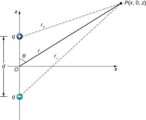
Now let us consider the special case when the distance of the point P from the dipole is much greater than the distance between the charges in the dipole, \(r >> d\); for example, when we are interested in the electric potential due to a polarized molecule such as a water molecule. This is not so far (infinity) that we tin simply care for the potential as cypher, just the altitude is great plenty that nosotros can simplify our calculations relative to the previous instance.
We starting time past noting that in Effigy \(\PageIndex{4}\) the potential is given by
\[V_p = V_+ + V_- = k \left( \dfrac{q}{r_+} - \dfrac{q}{r_-} \right)\]
where
\[r_{\pm} = \sqrt{x^two + \left(z \pm \dfrac{d}{2}\right)^2}.\]
This is still the exact formula. To take advantage of the fact that \(r \gg d\), we rewrite the radii in terms of polar coordinates, with \(10 = r \, \sin \, \theta\) and z = r \, \cos \, \theta\). This gives us
\[r_{\pm} = \sqrt{r^2 \, \sin^2 \, \theta + \left(r \, \cos \, \theta \pm \dfrac{d}{ii} \right)^ii}.\]
We can simplify this expression by pulling r out of the root,
\[r_{\pm} = \sqrt{\sin^ii \, \theta + \left(r \, \cos \, \theta \pm \dfrac{d}{ii} \correct)^2}\]
then multiplying out the parentheses
\[r_{\pm} = r \sqrt{\sin^2\space \theta + \cos^2 \, \theta \pm \cos \, \theta\dfrac{d}{r} + \left(\dfrac{d}{2r}\right)^2} = r\sqrt{ane \pm \cos \, \theta \dfrac{d}{r} + \left(\dfrac{d}{2r}\right)^2}.\]
The last term in the root is small enough to exist negligible (remember \(r >> d\), and hence \((d/r)^2\) is extremely pocket-sized, effectively goose egg to the level we will probably be measuring), leaving usa with
\[r_{\pm} = r\sqrt{1 \pm \cos \, \theta \dfrac{d}{r}}.\]
Using the binomial approximation (a standard result from the mathematics of series, when \(a\) is small)
\[\dfrac{1}{\sqrt{one \pm a}} \approx 1 \pm \dfrac{a}{2}\]
and substituting this into our formula for \(V_p\), we get
\[V_p = yard\left[\dfrac{q}{r}\left(1 + \dfrac{d \, \cos \, \theta}{2r} \right) - \dfrac{q}{r}\left(1 - \dfrac{d \, \cos \, \theta}{2r}\right)\right] = thousand\dfrac{qd \, \cos \theta}{r^2}.\]
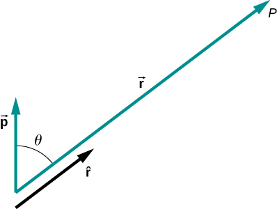
This may be written more conveniently if nosotros ascertain a new quantity, the electric dipole moment ,
\[\vec{p} = q\vec{d},\]
where these vectors point from the negative to the positive charge. Note that this has magnitude qd. This quantity allows us to write the potential at point P due to a dipole at the origin as
\[V_p = k\dfrac{\vec{p} \cdot \hat{r}}{r^two}.\]
A diagram of the application of this formula is shown in Figure \(\PageIndex{v}\).
There are also college-gild moments, for quadrupoles, octupoles, and so on. Yous will see these in future classes.
Potential of Continuous Charge Distributions
We have been working with point charges a great deal, but what nigh continuous charge distributions? Recall from Equation \ref{eq20} that
\[V_p = k\sum \dfrac{q_i}{r_i}.\]
We may treat a continuous charge distribution every bit a collection of infinitesimally separated private points. This yields the integral
\[V_p = \int \dfrac{dq}{r}\]
for the potential at a bespeak P. Notation that \(r\) is the distance from each individual bespeak in the charge distribution to the bespeak P. As nosotros saw in Electric Charges and Fields, the infinitesimal charges are given by
\[\underbrace{dq = \lambda \, dl}_{one \, dimension}\]
\[\underbrace{dq = \sigma \, dA}_{2 \, dimensions}\]
\[\underbrace{dq = \rho \, dV \space}_{three \, dimensions}\]
where \(\lambda\) is linear charge density, \(\sigma\) is the charge per unit area, and \(\rho\) is the charge per unit volume.
Case \(\PageIndex{4}\): Potential of a Line of Charge
Discover the electric potential of a uniformly charged, nonconducting wire with linear density \(\lambda\) (coulomb/meter) and length 50 at a point that lies on a line that divides the wire into two equal parts.
Strategy
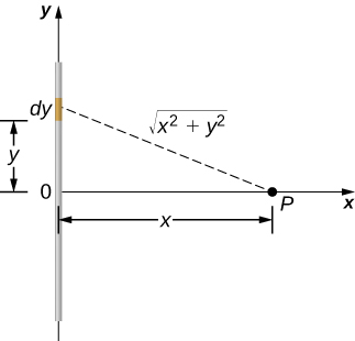
To set upward the trouble, we choose Cartesian coordinates in such a way every bit to exploit the symmetry in the problem every bit much equally possible. Nosotros place the origin at the middle of the wire and orient the y-axis forth the wire so that the ends of the wire are at \(y = \pm 50/2\). The field indicate P is in the xy-plane and since the choice of axes is up to us, we choose the ten-axis to pass through the field point P, equally shown in Effigy \(\PageIndex{6}\).
Solution
Consider a pocket-size element of the charge distribution betwixt y and \(y + dy\). The accuse in this cell is \(dq = \lambda \, dy\) and the distance from the cell to the field betoken P is \(\sqrt{x^2 + y^2}\). Therefore, the potential becomes
\[\begin{align} V_p &= k \int \dfrac{dq}{r} \nonumber \\[4pt] &= one thousand\int_{-Fifty/2}^{L/two} \dfrac{\lambda \, dy}{\sqrt{x^2 + y^ii}} \nonumber \\[4pt] &= k\lambda \left[ln \left(y + \sqrt{y^ii + x^2}\right) \right]_{-L/ii}^{50/2} \nonumber \\[4pt] &= yard\lambda \left[ ln \left(\left(\dfrac{Fifty}{two}\right) + \sqrt{\left(\dfrac{L}{2}\right)^2 + x^2}\right) - ln\left(\left(-\dfrac{L}{2}\right) + \sqrt{\left(-\dfrac{L}{2}\right)^ii + x^2}\correct)\correct] \nonumber \\[4pt] &= k\lambda ln \left[ \dfrac{L + \sqrt{L^2 + 4x^ii}}{-50 + \sqrt{L^2 + 4x^2}}\right]. \nonumber \end{marshal} \nonumber\]
Significance
Note that this was simpler than the equivalent problem for electric field, due to the utilise of scalar quantities. Retrieve that we expect the nothing level of the potential to be at infinity, when we have a finite accuse. To examine this, we take the limit of the above potential as x approaches infinity; in this case, the terms inside the natural log arroyo i, and hence the potential approaches zero in this limit. Annotation that we could have done this problem equivalently in cylindrical coordinates; the only effect would be to substitute r for ten and z for y.
Example \(\PageIndex{5}\): Potential Due to a Band of Charge
A band has a compatible charge density \(\lambda\), with units of coulomb per unit of measurement meter of arc. Find the electric potential at a point on the axis passing through the centre of the band.
Strategy
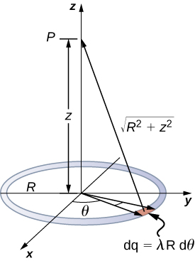
We employ the aforementioned procedure every bit for the charged wire. The deviation here is that the charge is distributed on a circumvolve. Nosotros divide the circle into infinitesimal elements shaped as arcs on the circle and use cylindrical coordinates shown in Figure \(\PageIndex{seven}\).
Solution
A general chemical element of the arc between \(\theta\) and \(\theta + d\theta\) is of length \(Rd\theta\) and therefore contains a charge equal to \(\lambda Rd\theta\). The element is at a distance of \(\sqrt{z^2 + R^ii}\) from P, and therefore the potential is
\[\begin{marshal} V_p &= k\int \dfrac{dq}{r} \nonumber \\[4pt] &= k \int_0^{2\pi} \dfrac{\lambda Rd\theta}{\sqrt{z^two + R^ii}} \nonumber \\[4pt] &= \dfrac{m \lambda R}{\sqrt{z^ii + R^2}} \int_0^{two\pi} d\theta \nonumber \\[4pt] &= \dfrac{two\pi k \lambda R}{\sqrt{z^two + R^2}} \nonumber \\[4pt] &= one thousand \dfrac{q_{tot}}{\sqrt{z^2 + R^2}}. \nonumber \end{align} \nonumber\]
Significance
This result is expected because every element of the ring is at the same distance from indicate P. The net potential at P is that of the total charge placed at the common distance, \(\sqrt{z^2 + R^2}\).
Case \(\PageIndex{6}\): Potential Due to a Uniform Disk of Charge
A disk of radius R has a uniform charge density \(\sigma\) with units of coulomb meter squared. Find the electrical potential at whatever point on the axis passing through the center of the disk.
Strategy
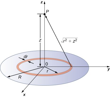
Nosotros split up the disk into ring-shaped cells, and make employ of the upshot for a ring worked out in the previous example, so integrate over r in addition to \(\theta\). This is shown in Figure \(\PageIndex{8}\).
Solution
An infinitesimal width cell between cylindrical coordinates r and \(r + dr\) shown in Effigy \(\PageIndex{viii}\) will be a band of charges whose electrical potential \(dV_p\) at the field bespeak has the post-obit expression
\[dV_p = 1000 \dfrac{dq}{\sqrt{z^2 + r^ii}}\]
where
\[dq = \sigma 2\pi r dr.\]
The superposition of potential of all the minute rings that make up the deejay gives the net potential at point P. This is achieved by integrating from \(r = 0\) to \(r = R\):
\[\begin{align} V_p &= \int dV_p = k2\pi \sigma \int_0^R \dfrac{r \, dr}{\sqrt{z^2 + r^2}}, \nonumber \\[4pt] &= k2\pi \sigma ( \sqrt{z^2 + R^two} - \sqrt{z^2}).\nonumber \end{align} \nonumber\]
Significance
The basic procedure for a deejay is to showtime integrate around θ and then over r. This has been demonstrated for uniform (constant) accuse density. Often, the accuse density will vary with r, and then the last integral will requite different results.
Example \(\PageIndex{7}\): Potential Due to an Infinite Charged Wire
Notice the electric potential due to an infinitely long uniformly charged wire.
Strategy
Since we take already worked out the potential of a finite wire of length 50 in Example \(\PageIndex{4}\), we might wonder if taking \(Fifty \rightarrow \infty\) in our previous result will work:
\[V_p = \lim_{L \rightarrow \infty} 1000 \lambda \ln \left(\dfrac{50 + \sqrt{L^ii + 4x^2}}{-L + \sqrt{L^ii + 4x^2}}\right).\]
Notwithstanding, this limit does non exist because the argument of the logarithm becomes [ii/0] every bit \(Fifty \rightarrow \infty\), so this way of finding V of an space wire does non work. The reason for this problem may be traced to the fact that the charges are not localized in some space but keep to infinity in the management of the wire. Hence, our (unspoken) assumption that zero potential must exist an infinite distance from the wire is no longer valid.
To avert this difficulty in calculating limits, allow united states of america apply the definition of potential past integrating over the electric field from the previous section, and the value of the electric field from this charge configuration from the previous affiliate.
Solution
Nosotros use the integral
\[V_p = - \int_R^p \vec{Due east} \cdot d\vec{fifty}\]
where R is a finite altitude from the line of accuse, as shown in Figure \(\PageIndex{ix}\).
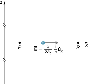
With this setup, we utilise \(\vec{E}_p = 2k \lambda \dfrac{1}{south} \hat{s}\) and \(d\vec{fifty} = d\vec{s}\) to obtain
\[\begin{marshal} V_p - V_R &= - \int_R^p 2k\lambda \dfrac{1}{s}ds \nonumber \\[4pt] &= -ii one thousand \lambda \ln\dfrac{s_p}{s_R}. \nonumber \end{marshal} \nonumber\]
Now, if we define the reference potential \(V_R = 0\) at \(s_R = one \, m\), this simplifies to
\[V_p = -2 k\lambda \, \ln \, s_p.\]
Note that this form of the potential is quite usable; information technology is 0 at 1 m and is undefined at infinity, which is why we could not apply the latter every bit a reference.
Significance
Although calculating potential directly can be quite convenient, we just constitute a arrangement for which this strategy does not piece of work well. In such cases, going dorsum to the definition of potential in terms of the electric field may offer a way forward.
Exercise \(\PageIndex{seven}\)
What is the potential on the axis of a nonuniform band of charge, where the charge density is \(\lambda (\theta) = \lambda \, \cos \, \theta\)?
Solution
It will exist nix, as at all points on the axis, in that location are equal and opposite charges equidistant from the point of interest. Note that this distribution will, in fact, have a dipole moment.
Source: https://phys.libretexts.org/Bookshelves/University_Physics/Book%3A_University_Physics_(OpenStax)/Book%3A_University_Physics_II_-_Thermodynamics_Electricity_and_Magnetism_(OpenStax)/07%3A_Electric_Potential/7.04%3A_Calculations_of_Electric_Potential
0 Response to "what is the potential v0 in the limit as h goes to zero?"
Post a Comment